3  Markdown, project workflows

3.1 Lesson preamble

3.1.1 Lesson objectives

• Learn about the Markdown syntax and how to use it within the R Notebook.
• Set up the R Notebook
• Set up an R Project
• Understand how to follow the conventional data science workflow

3.1.2 Learning outline

• Explore RStudio interface (10 mins)
• Reproducible science with Markdown (40 mins)
• Project-Oriented Workflow (20 mins)
• Reproducible Science (10 mins)
• The Scientific Method (10 mins)
• Find your groups! (10 mins)

---

3.2 Markdown

Last class, we introduced Markdown, the text format that RStudio uses. In fact, if you are following along this far, you should have already been typing your notes and code in a .Rmd file, or a RMarkdown file.

Let’s introduce more Markdown features! We encourage groups to try completing their group projects in RMarkdown, but more about that later.

3.2.1 In-line code

We talked about using RMarkdown for notes and inline code last class. This is extremely useful for when you need to update objects or rerun analyses. You can also comment out code within the code chunk.

As a reminder, the keyboard shortcut to insert a code chunk is:

• command + option + i (Mac)
• ctrl + alt + i (Windows)

x <- 5
y <- 13

# 5 plus 13
x + y

[1] 18

3.2.1.1 R code chunk tricks

• eval=TRUE evaluates the code chunk (runs it); eval=FALSE does not (will just print the chunk)
• echo=TRUE prints the code chunk; echo=FALSE hides it but will still evaluate it
  • this is useful if you need to save something as an object but you don’t necessarily need it to print
• warning=FALSE will hide warnings; message=FALSE will hide messages from output
  • only the case when eval=TRUE

## eval=TRUE, echo=FALSE prints output, but does not print code chunk
library(ggplot2)
qplot(mpg, wt, data = mtcars)

Warning: `qplot()` was deprecated in ggplot2 3.4.0.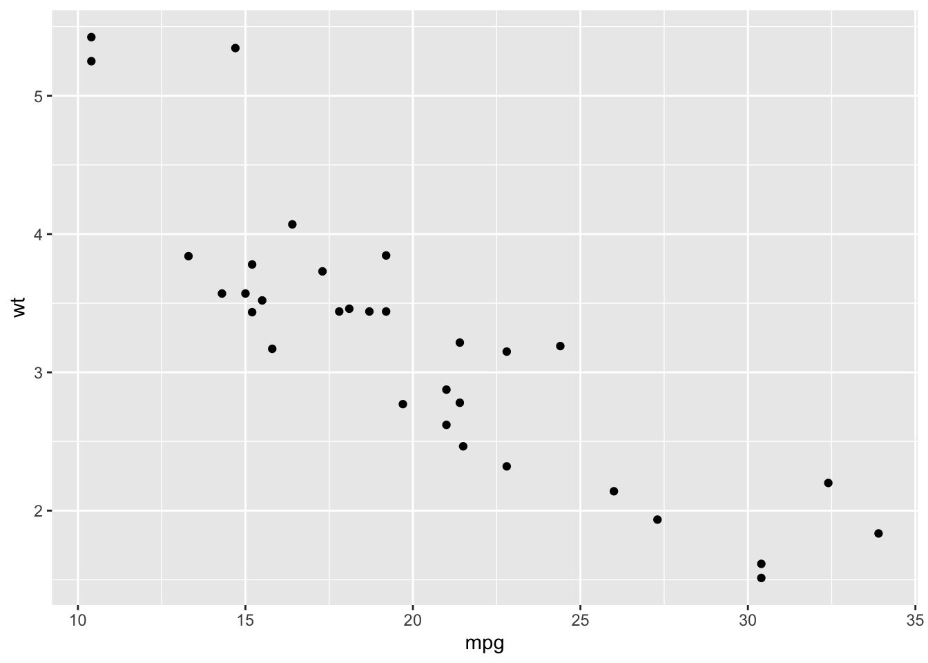

3.2.1.2 Changing height and width of images/figures

You can also indicate the sizes of figures by using fig.width and fig.height in your code chunk.

## in this R chuck, fig.width=2, fig.height=2
qplot(mpg, wt, data = mtcars)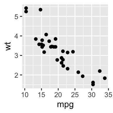

3.2.2 Lists

I’ve already used these! You can use either * or - to indicate unordered lists. To indent, hit tab. Make sure there’s a space before your items in the list.

Unordered Lists (bullet points)

• first item
• second item
  • sub-level item (two tabs)
• third item

For ordered lists, use numbers. Again, hit tab to add sublists.

Ordered Lists (numbers)

1. Ordered item
2. Ordered item
   1. Ordered sub-item
3. Item (will automatically re-number)

3.2.3 Tables

kable displays r code chunks with tables nicely

library(knitr)
kable(head(mtcars))

	mpg	cyl	disp	hp	drat	wt	qsec	vs	am	gear	carb
Mazda RX4	21.0	6	160	110	3.90	2.620	16.46	0	1	4	4
Mazda RX4 Wag	21.0	6	160	110	3.90	2.875	17.02	0	1	4	4
Datsun 710	22.8	4	108	93	3.85	2.320	18.61	1	1	4	1
Hornet 4 Drive	21.4	6	258	110	3.08	3.215	19.44	1	0	3	1
Hornet Sportabout	18.7	8	360	175	3.15	3.440	17.02	0	0	3	2
Valiant	18.1	6	225	105	2.76	3.460	20.22	1	0	3	1

In comparison:

library(knitr)
head(mtcars) ## does not nicely format the table

               mpg cyl disp  hp drat    wt  qsec vs am gear carb

Mazda RX4 21.0 6 160 110 3.90 2.620 16.46 0 1 4 4 Mazda RX4 Wag 21.0 6 160 110 3.90 2.875 17.02 0 1 4 4 Datsun 710 22.8 4 108 93 3.85 2.320 18.61 1 1 4 1 Hornet 4 Drive 21.4 6 258 110 3.08 3.215 19.44 1 0 3 1 Hornet Sportabout 18.7 8 360 175 3.15 3.440 17.02 0 0 3 2 Valiant 18.1 6 225 105 2.76 3.460 20.22 1 0 3 1

3.2.4 Images and Links

Use the following format to add images:

![Description/Caption](/path/to/image.png)

For example:

As an aside, let’s talk about rubber duck debugging. It is a simple but effective technique used by scientists to debug code. By explaining the code line-by-line to an inanimate object, such as a rubber duck, programmers can break down the code into smaller, more manageable pieces, and potentially identify the root cause of the problem. Or, explain it to a friend in the course! They can also help you find typos and other errors

And use the following format to add weblinks: [Description/Caption](weblink).

The EEB website lives here!

3.2.5 White Space and New Page

Use \vspace{2pt} to add white space, and use \newpage to add a page break.

3.2.6 In-line citations and bibliography

Export a .bib file (e.g., from Zotero and Mendeley). Then, add the .bib to your YAML header.

---
title: My Report
output: html_document
bibliography: bibliography.bib
---

Now, you can cite directly in your report, like below:

Some fact[@Smith2018]

Some fact supported by multiple papers [@Smith2018; @Tran1997]

3.2.7 Footnotes

This is what a footnote looks like.¹ Here is another.²

3.3 Project-Oriented Workflow

3.3.1 Projects

Material adapted from Posit and R-bloggers.

RStudio projects make it straightforward to divide your work into multiple contexts, each with their own working directory, workspace, history, and source documents.

To create a new project in the RStudio IDE, use the Create Project command (top right). You can link your new project to an existing directory, or create a new directory entirely. Since we already have some RMarkdown written, let’s add our project to an existing directory.

When a new project is created RStudio, it creates a project file (with an .Rproj extension) within the project directory. This file contains various project options (discussed below) and can also be used as a shortcut for opening the project directly from the filesystem. It also creates a hidden directory (named .Rproj.user) where project-specific temporary files (e.g., auto-saved source documents, window-state, etc.) are stored. This directory is also automatically added to .Rbuildignore, .gitignore, etc. if required.

Now, whenever you open your project, it loads your project into RStudio and displays its name in the Projects toolbar (which is located on the far right side of the main toolbar). It even takes you back to where you were working last, so it opens all the scripts and files that were last open! You can also save your history, the objects in your environment, and an image of what your project looked like at the last time you closed it, but this can take up a lot of space if you do this each time.

You can work with more than one RStudio project at a time by simply opening each project in its own window of RStudio.

3.3.2 Relative File Pathways

The goal of the here package is to enable easy file referencing in project-oriented workflows. In contrast to using setwd(), which is fragile and dependent on the way you organize your files, here uses the top-level directory of a project to easily build paths to files.

library(here)

here() starts at /Users/vicki.zhang/Documents/UofT/PhD/Teaching/2023-2024/eeb313.github.io

here()

[1] "/Users/vicki.zhang/Documents/UofT/PhD/Teaching/2023-2024/eeb313.github.io"

You can build a path relative to the top-level directory in order to read or write a file:

here("1_lectures", "csv", "portal_data.csv")

[1] "/Users/vicki.zhang/Documents/UofT/PhD/Teaching/2023-2024/eeb313.github.io/1_lectures/csv/portal_data.csv"

These relative paths work regardless of where the associated source file lives inside your project, like analysis projects with data and reports in different subdirectories.

3.3.3 Demo Project

There is no a single “right” folder structure for analysis projects. However, this is a tried-and-true simple method that works (backed up by many data scientists!).

Create a folder on your computer that holds all the files relevant to that particular piece of work. This parent folder will contain the project’s .Rproj and all other subfolders, so it should have the same name as your project. Pick a good one. Spending an extra 5 minutes will save you from regrets in the future. The name should be short, concise, written in lower-case, and not containing any special symbols. One can apply similar strategies as for naming packages.

Use subdirectories to organize data, code, figures, notes, etc.

• The folder data typically contains two subfolders, namely, raw and processed. The content of raw directory is data files of any kind, such as .csv, SAS, Excel, text and database files, etc. The content of this folder is read-only, so that no scripts should change the original files or create new ones inside it. For this purpose, the processed directory is used: all processed, cleaned, and tidied datasets are saved here. It is a good practice to save files in R specific format, rather than in .csv, since the saving in .csv is a less efficient way of storing data (both in terms of space and time of reading/writing).
• The folder figures is the place where you may store plots, diagrams, and other figures. There is not much to say about it. Common extensions of such files are .eps, .png, .pdf, etc. Again, file names in this folder should be meaningful (the name img1.png does not represent anything).
• All reports live in a directory with the corresponding name reports. These reports can be of any formats, such as LaTeX, Markdown, R Markdown, Jupyter Notebooks, etc. Currently, more and more people prefer rich documents with text and executable code to LaTeX and such.
• Perhaps the most important folder is analyses or scripts. Here, you keep all your R scripts and codes. That is the exact place to use prefix numbers, if files should be run in a particular order. If you have files in other scripted languages (e.g., Python), it is better to keep them in this folder as well. There can also an important subfolder called deprecated. Whenever you want to remove one or the other script, it is a good idea to move it to deprecated at first iteration. I recommend never deleting your code until you are sure that you have finished everything you wanted to do, even if the code doesn’t work (going back to it after a break usually helps!).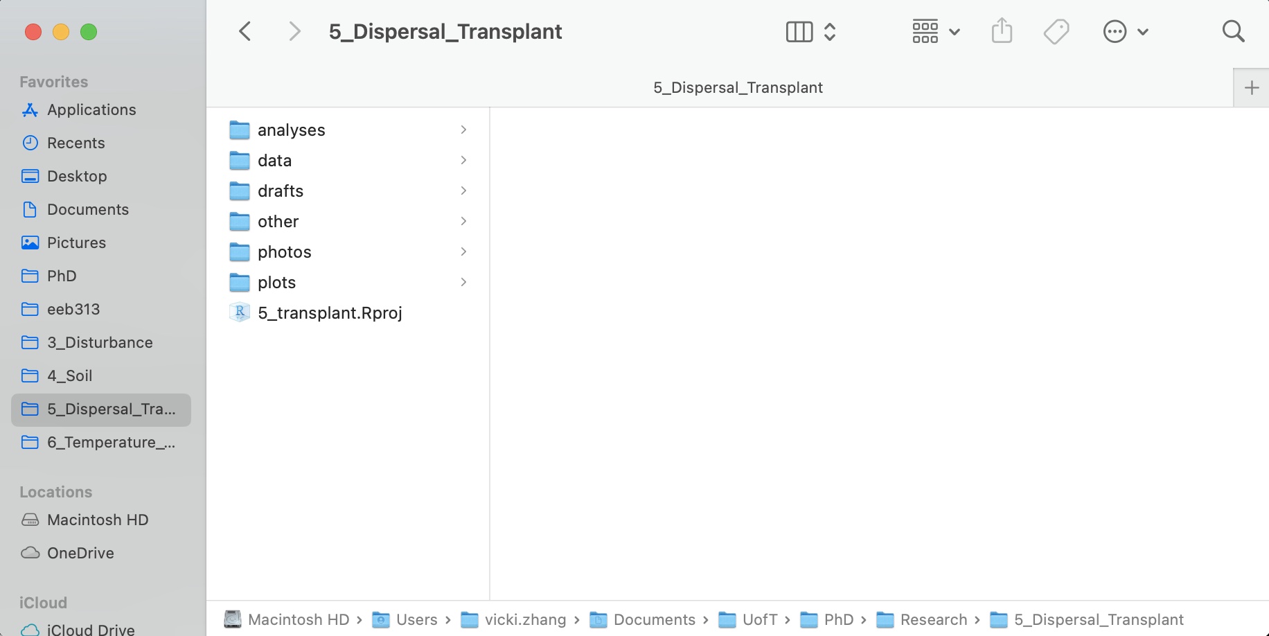

Vicki’s demo of her file directory.

This convention guarantees that the project is self-contained, and it can be moved around on your computer or onto other computers and will still “just work”. This is a really important convention that creates reliable, reproducible science across different computers or users and over time.

3.3.4 Documenting session info

As an overview of our environment, we can also use the sessionInfo() command. This is a good practice to have at the end of your code to document which packages you used and what version they were.

sessionInfo()

R version 4.1.1 (2021-08-10)
Platform: x86_64-apple-darwin17.0 (64-bit)
Running under: macOS Big Sur 10.16

Matrix products: default
BLAS:   /Library/Frameworks/R.framework/Versions/4.1/Resources/lib/libRblas.0.dylib
LAPACK: /Library/Frameworks/R.framework/Versions/4.1/Resources/lib/libRlapack.dylib

locale:
[1] en_CA.UTF-8/en_CA.UTF-8/en_CA.UTF-8/C/en_CA.UTF-8/en_CA.UTF-8

attached base packages:
[1] stats     graphics  grDevices utils     datasets  methods   base     

other attached packages:
[1] here_1.0.1    knitr_1.44    ggplot2_3.4.3

loaded via a namespace (and not attached):
 [1] rstudioapi_0.15.0 magrittr_2.0.3    tidyselect_1.2.0  munsell_0.5.0    
 [5] colorspace_2.1-0  R6_2.5.1          rlang_1.1.1       fastmap_1.1.1    
 [9] fansi_1.0.4       dplyr_1.1.3       tools_4.1.1       grid_4.1.1       
[13] gtable_0.3.4      xfun_0.40         utf8_1.2.3        cli_3.6.1        
[17] withr_2.5.1       htmltools_0.5.6   rprojroot_2.0.3   digest_0.6.33    
[21] tibble_3.2.1      lifecycle_1.0.3   farver_2.1.1      htmlwidgets_1.6.2
[25] vctrs_0.6.3       glue_1.6.2        evaluate_0.21     rmarkdown_2.25   
[29] labeling_0.4.3    compiler_4.1.1    pillar_1.9.0      generics_0.1.3   
[33] scales_1.2.1      jsonlite_1.8.7    pkgconfig_2.0.3  

Notice that we have some base packages active even though we did not explicitly call for them.

3.4 Reproducible Science

• Computational reproducibility
  • code, software, etc.
• Scientific reproducibility
  • data (able to run the same statistical analysis on the same data)
  • method, details about how the data was collected
  • N.B., field work - hard to reproduce method
• Statistical reproducibility

1. Why does reproducibility matter in science?
   • Must trust findings to build on scientific progress!
2. What do you think about when you hear the term “open science”?
   • Open science: everything about a project (data, stats, code, funding, etc.) is open and available to viewing
3. How does open science affect collaboration and the progress of science?

What are the barriers to reproducibility?

• people won’t care
• people might want to steal results
• researchers do not want to share (embarrassed, code is rushed, etc.)

3.4.1 Reproducibility in Data Science

Material from this section adapted from R for Data Science.

The main tools of data science are: importing, tidying, transforming, and visualizing data. We will go through all of these steps of data science so that you can tackle real datasets.

Data Science Workflow

1. Before you can transform and visualize your data, you need to first get your data into R.
2. Then, you’ll learn about tidy data, a consistent way of storing your data that makes transformation, visualization, and modelling easier. You’ll learn the underlying principles, and how to get your data into a tidy form.
3. You’ll learn the key verbs that allow you to select important variables, filter out key observations, create new variables, and compute summaries.
4. Finally, we will visualize by making elegant and informative plots that help you understand data.

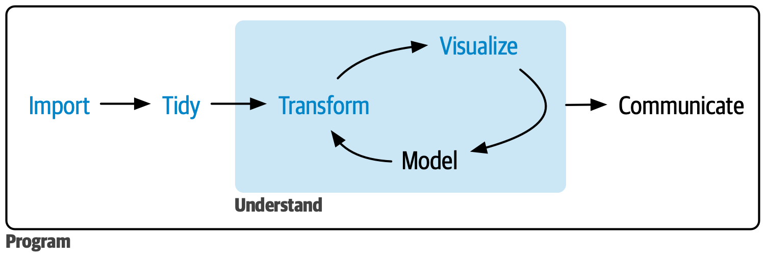
Note that if you are interested in doing a modelling project, these steps are different. Talk to Vicki and Mete if you want to tackle mathematical models!

3.5 The Scientific Method

3.5.1 Steps in scientific process

1. Identify research question(s).
2. Look into what the previous literature shows.
3. Create one or more hypotheses or objectives.
4. Write up an outline or expected approach to answering those questions/objectives (analysis and presentation plan):

• How will the data be obtained and what is the data (i.e. the source)?
• What statistical/mathematical techniques have previous researchers used? Will you use them? Are they appropriate (optional, may need expert)? ( How will the results/data be presented or visualized (possible tables/figures)?

5. Run the planned analyses (or additional ones that come may up).
6. Visualize or present all results from the analyses.
7. Interpret the results and how they fit with the previous literature.
8. Draw conclusions based on the hypotheses/objectives.
9. Disseminate your results (in blogs, pre-print archives, journals, conferences)

Simplified diagram of the scientific method

3.5.2 Basics of succeeding as a team

Final assignment is in a group and to succeed, you need to understand team dynamics:

• Communication is vital to work together and to achieve the goal
• Teams go through various stages
• Need consensus for group norms, goals, duties/responsibilities, and conduct/behaviour
• Important that everyone has a stake in the project
• Rotate roles (specifically for the leader/facilitator)

3.5.3 Roles and responsibilities

• Leader/Facilitator’s duty:
  • Goal is to keep things running smoothly, focused on the task, and on track for time
  • Keep everyone on topic and on task; stay aware of the time
  • (Try to) mediate or resolve any conflicts (there will always be some type of conflict; how it’s dealt with is what matters)
  • (Try to) encourage everyone to participate and allow everyone a chance at talking
• Recorder’s duty:
  • Goal is to write/type down main or important points raised or discussed when team is meeting
  • Keep notes and files organized and orderly
• Organizer’s duty:
  • Arrange for next meeting time and location
• Send reminders to members a day or two before meeting
  • Make and email a simple agenda of tasks to do or to discuss

3.5.4 Code of Conduct

• Vital to establishing boundaries and expectations of being a team member
  • How do you want each member to treat each other?
  • How do you deal with conflict?
  • What is acceptable and unacceptable behaviour?
• These are outlined in the code of conduct
• Mostly its common sense (be kind and respectful)
  • But its important that you as a team write out what everyone wants and agrees to

3.5.4.1 Example Code of Conduct

Check out the Contributor Convenent and the UofT Coders Code of Conduct

3.6 Projects!

3.6.1 Exercise after groups are formed

As a group, complete these tasks:

1. Get into your groups
2. Introduce one another:

• Name, year of study
• Other stuff (e.g., interests, plans for next years, etc.)

3. Create a “team name”
4. Assign roles to each other:

• These will be rotated: Leader/Facilitator, Recorder, Organizer
• Discuss how and when the roles will be rotated.

5. Discuss and brainstorm code of conduct (record it).
6. Take a minute to think about your own skills

• Share these with your group (record them).

7. Discuss how responsibilities of each member will be decided on (record it).

3.6.2 GitHub

Make a GitHub account.

---

1. This is the first footnote.

2. This is the second footnote.